Using Machine Learning Algorithm for Predicting House Valuations

Machine learning has been used for years to offer image recognition, spam detection, natural speech comprehension, product recommendations, and medical diagnoses. Today, machine learning algorithms can help us enhance cybersecurity, ensure public safety, and improve medical outcomes. Machine learning systems can also make customer service better and automobiles safer.

When I started experimenting with machine learning, I wanted to come up with an application that would solve a real-world problem but would not be too complicated to implement. I also wanted to practice working with regression algorithms. So I started looking for a problem worth solving. Here’s what I came up with.

If you’re going to sell a house, you need to know what price tag to put on it. And a computer algorithm can give you an accurate estimate!

In this article, I’ll show you how I wrote a regression algorithm to predict home prices.

Regression in a nutshell

Put simply, regression is a machine learning tool that helps you make predictions by learning – from the existing statistical data – the relationships between your target parameter and a set of other parameters. According to this definition, a house’s price depends on parameters such as the number of bedrooms, living area, location, etc. If we apply artificial learning to these parameters we can calculate house valuations in a given geographical area.

The idea of regression is pretty simple: given enough data, you can observe the relationship between your target parameter (the output) and other parameters (the input), and then apply this relationship function to real observed data.

To show you how regression algorithm works we’ll take into account only one parameter – a home’s living area – to predict price. It’s logical to suppose that there is a linear relationship between area and price. And as we remember from high school, a linear relationship is represented by a linear equation:

y = k0 + k1*x

In our case, y equals price and x equals area. Predicting the price of a home is as simple as solving the equation (where k0 and k1 are constant coefficients):

price = k0 + k1 * area

We can calculate these coefficients (k0 and k1) using regression. Let’s assume we have 1000 known house prices in a given area. Using a learning technique, we can find a set of coefficient values. Once found, we can plug in different area values to predict the resulting price.

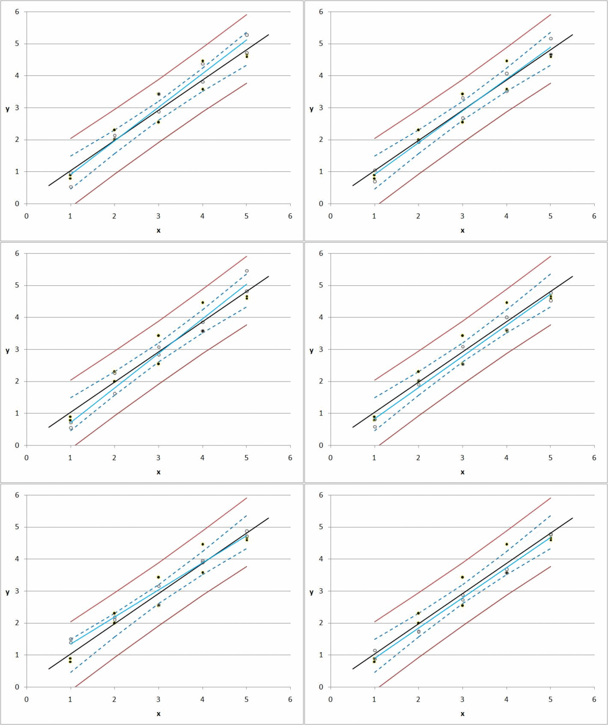
[In this graph, y is price and x is living area. Black dots are our observations. Moving lines show what happens when k0 and k1 change.]

But there is always a deviation, or difference between a predicted value and an actual value. If we have 1000 observations, then we can calculate the total deviation of all items by summing the deviations for each k0 and k1 combination.

Regression takes every possible value for k0 and k1 and minimizes the total deviation; this is the idea of regression in a nutshell.

But in real life, there are other challenges you need to deal with. House prices obviously depend on multiple parameters, and there is no clear linear relationship between all of these parameters.

Now I’m going to tell you how I used regression algorithms to predict house price for my pet project.

How to use regression algorithms in machine learning

1. Gather data

The first step for any kind of machine learning analysis is gathering the data – which must be valid. If you can’t guarantee the validity of your data, then there’s no point analyzing it. You need to pay attention to the source you take your data from.

For my purposes, I’ve relied on a database from one of the largest real-estate portals in the Netherlands. Since the real estate market in the Netherlands is strictly regulated, I didn’t have to check its validity.

Initially I had to do some data mining because the required data were available in various formats across multiple sources. In most real-world projects you’ll have to do some data mining as well. We won’t discuss data mining here, however, as it’s not really relevant to our topic.

For the purpose of this article, let’s imagine that all the real-estate data I found were in the format shown below.

2. Analyze data

Once you’ve gathered data it’s time to analyze it. After parsing the data I got the following records:

{ "has_garden" : 1, "year" : 1980, "lng" : 4.640685, "has_garage" : 0, "changes_count" : "2", "area" : 127, "bedrooms_count" : "4", "com_time" : 57, "price" : 305000, "energy_label" : 1, "lat" : 52.30177, "rooms_count" : "5", "life_quality" : 6, "house_type" : 1, "is_leasehold" : 0 }
{ "has_garden" : 1, "year" : 1980, "lng" : 4.656503, "has_garage" : 0, "changes_count" : "3", "area" : 106, "bedrooms_count" : "3", "com_time" : 64, "price" : 275000, "energy_label" : 3, "lat" : 52.35456, "rooms_count" : "4", "life_quality" : 5, "house_type" : 1, "is_leasehold" : 0 }
{ "has_garden" : 1, "year" : 1980, "lng" : 4.585596, "has_garage" : 0, "changes_count" : "3", "area" : 106, "bedrooms_count" : "3", "com_time" : 74, "price" : 244000, "energy_label" : 3, "lat" : 52.29309, "rooms_count" : "4", "life_quality" : 6, "house_type" : 1, "is_leasehold" : 0 }
{ "has_garden" : 1, "year" : 1980, "lng" : 4.665817, "has_garage" : 0, "changes_count" : "2", "area" : 102, "bedrooms_count" : "4", "com_time" : 77, "price" : 199900, "energy_label" : 3, "lat" : 52.14919, "rooms_count" : "5", "life_quality" : 6, "house_type" : 1, "is_leasehold" : 0 }
{ "has_garden" : 1, "year" : 1980, "lng" : 4.620336, "has_garage" : 0, "changes_count" : "1", "area" : 171, "bedrooms_count" : "3", "com_time" : 79, "price" : 319000, "energy_label" : 1, "lat" : 52.27822, "rooms_count" : "4", "life_quality" : 6, "house_type" : 1, "is_leasehold" : 0 }
{ "has_garden" : 1, "year" : 1980, "lng" : 5.062804, "has_garage" : 1, "changes_count" : "1", "area" : 139, "bedrooms_count" : "5", "com_time" : 38, "price" : 265000, "energy_label" : 5, "lat" : 52.32992, "rooms_count" : "6", "life_quality" : 7, "house_type" : 1, "is_leasehold" : 0 }
{ "has_garden" : 1, "year" : 1980, "lng" : 5.154957, "has_garage" : 1, "changes_count" : "2", "area" : 129, "bedrooms_count" : "4", "com_time" : 57, "price" : 309500, "energy_label" : 1, "lat" : 52.35634, "rooms_count" : "5", "life_quality" : 6, "house_type" : 1, "is_leasehold" : 0 }
{ "has_garden" : 1, "year" : 1980, "lng" : 4.622486, "has_garage" : 0, "changes_count" : "1", "area" : 125, "bedrooms_count" : "4", "com_time" : 76, "price" : 289000, "energy_label" : 1, "lat" : 52.2818, "rooms_count" : "5", "life_quality" : 6, "house_type" : 1, "is_leasehold" : 0 }

Here’s what the fields mean:

has_garden – does the property has a garden? 1 – true, 0 – false
year – year of construction
lat, lng – house location coordinates
area – total living area
has_garage – does the property has a garage? 1 – true, 0 – false
bedrooms_count – amount of bedrooms
rooms_count – total rooms count
energy_label – energy efficiency label (assigned for each house in the Netherlands)
life_quality – life quality mark calculated for each district by local authorities
house_type – property type (1 – house, 0 – appartement)
com_time – commuting time to Amsterdam center
changes_count – transport changes count if you go to Amsterdam center by public transport

I worked on the assumption that these are all measurable data that affect a home’s price. Of course, there may be more parameters that matter as well, such as house condition and location. But these parameters are more subjective and almost impossible to measure, so I ignored them.

3. Check the correlation between parameters

Now you need to check for strong correlations among given parameters. If there are, then remove one of the parameters. In my dataset there were no strong correlations among values.

4. Remove outliers from the dataset

Outliers are observation points that are distant from other observations. For example, in my data there was one house with an area of 50 square meters for a price of $500K. Such houses may exist on the market for various reasons, but they are not statistically meaningful. I want to make a price estimate based on the market average, and so I won’t take such outliers into account.

Most regression methods explicitly require outliers be removed from the dataset as they may significantly affect the results. To remove the outlier I used the following function:

def get_outliners(dataset, outliers_fraction=0.25):
clf = svm.OneClassSVM(nu=0.95 * outliers_fraction + 0.05, kernel="rbf", gamma=0.1)
clf.fit(dataset)
result = clf.predict(dataset)
return result

This will return – 1 for outliers and 1 for non-outliers. Then you can do something like this:

training_dataset = full_dataset[get_outliners(full_dataset[analytics_fields_with_price], 0.15)==1]

After that you will have non-outlier observations only. Now it’s time to start regression analysis.

5. Choose a regression algorithm

There’s more than one way to do regression analysis. What we’re looking for is the best prediction accuracy given our data. But how can we check accuracy? A common way is to calculate a so-called r^2 score which is basically a squared difference between an actual and a predicted value.

It’s important to remember that if we use that same dataset for learning and checking our accuracy, our model may overfit. This means it will show excellent accuracy on a given dataset but will completely fail when given new data.

A common approach to solve this problem is to split the original dataset into two parts and then use one for learning and another for testing. This way we will simulate new data for our learning model, and if there is an overfit, we can spot it.

We can split our dataset using a proportion of 80/20. We’ll use 80% for training and the remaining 20% for testing. Let’s take a look at this piece of code:

//code for algorithm quality estimation

from sklearn import svm
import matplotlib.pyplot as plt
from sklearn.neighbors import KNeighborsRegressor
from sklearn.linear_model import LinearRegression, LogisticRegression
from sklearn.svm import SVR
from sklearn.metrics import r2_score
from sklearn.cross_validation import train_test_split
from sklearn.ensemble import RandomForestRegressor
import pandas as pd
 
    #prepare dataset  
    #....   
    #spilt dataset
    Xtrn, Xtest, Ytrn, Ytest = train_test_split(training_dataset[analytics_fields], training_dataset[['price']],
                                                test_size=0.2)
 
    # model = RandomForestRegressor(n_estimators=150, max_features='sqrt', n_jobs=-1)  # случайный лес
    models = [LinearRegression(),
              RandomForestRegressor(n_estimators=100, max_features='sqrt'),
              KNeighborsRegressor(n_neighbors=6),
              SVR(kernel='linear'),
              LogisticRegression()
              ]
 
    TestModels = pd.DataFrame()
    tmp = {}
 
    for model in models:
        # get model name
        m = str(model)
        tmp['Model'] = m[:m.index('(')]
        # fit model on training dataset
        model.fit(Xtrn, Ytrn['price'])
        # predict prices for test dataset and calculate r^2
        tmp['R2_Price'] = r2_score(Ytest['price'], model.predict(Xtest))
        # write obtained data
        TestModels = TestModels.append([tmp])
 
    TestModels.set_index('Model', inplace=True)
 
    fig, axes = plt.subplots(ncols=1, figsize=(10, 4))
    TestModels.R2_Price.plot(ax=axes, kind='bar', title='R2_Price')
    plt.show()

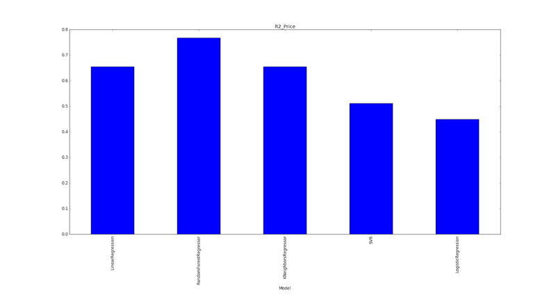
As a result, I got the following graph: